Algorithms
Table of Contents
- 1. Lecture 1
- 2. Lecture 2
- 3. Lecture 3
- 4. Lecture 4
- 5. Lecture 5
- 6. Lecture 6
- 7. Lecture 7
- 8. Lecture 8
1. Lecture 1
1.1. Data structure and Algorithm
- A data structure is a particular way of storing and organizing data. The purpose is to effectively access and modify data effictively.
- A procedure to solve a specific problem is called Algorithm.
During programming we use data structures and algorithms that work on that data.
1.2. Characteristics of Algorithms
An algorithm has follwing characteristics.
- Input : Zero or more quantities are externally supplied to algorithm.
- Output : An algorithm should produce atleast one output.
- Finiteness : The algorithm should terminate after a finite number of steps. It should not run infinitely.
- Definiteness : Algorithm should be clear and unambiguous. All instructions of an algorithm must have a single meaning.
- Effectiveness : Algorithm must be made using very basic and simple operations that a computer can do.
- Language Independance : A algorithm is language independent and can be implemented in any programming language.
1.3. Behaviour of algorithm
The behaviour of an algorithm is the analysis of the algorithm on basis of Time and Space.
- Time complexity : Amount of time required to run the algorithm.
- Space complexity : Amount of space (memory) required to execute the algorithm.
The behaviour of algorithm can be used to compare two algorithms which solve the same problem.
The preference is traditionally/usually given to better time complexity. But we may need to give preference to better space complexity based on needs.
1.3.1. Best, Worst and Average Cases
The input size tells us the size of the input given to algorithm. Based on the size of input, the time/storage usage of the algorithm changes. Example, an array with larger input size (more elements) will taken more time to sort.
- Best Case : The lowest time/storage usage for the given input size.
- Worst Case : The highest time/storage usage for the given input size.
- Average Case : The average time/storage usage for the given input size.
1.3.2. Bounds of algorithm
Since algorithms are finite, they have bounded time taken and bounded space taken. Bounded is short for boundries, so they have a minimum and maximum time/space taken. These bounds are upper bound and lower bound.
- Upper Bound : The maximum amount of space/time taken by the algorithm is the upper bound. It is shown as a function of worst cases of time/storage usage over all the possible input sizes.
- Lower Bound : The minimum amount of space/time taken by the algorithm is the lower bound. It is shown as a function of best cases of time/storage usage over all the possible input sizes.
1.4. Asymptotic Notations
1.4.1. Big-Oh Notation [O]
- The Big Oh notation is used to define the upper bound of an algorithm.
- Given a non negative funtion f(n) and other non negative funtion g(n), we say that \(f(n) = O(g(n)\) if there exists a positive number \(n_0\) and a positive constant \(c\), such that \[ f(n) \le c.g(n) \ \ \forall n \ge n_0 \]
- So if growth rate of g(n) is greater than or equal to growth rate of f(n), then \(f(n) = O(g(n))\).
2. Lecture 2
2.1. Asymptotic Notations
2.1.1. Omega Notation [ \(\Omega\) ]
- It is used to shown the lower bound of the algorithm.
- For any positive integer \(n_0\) and a positive constant \(c\), we say that, \(f(n) = \Omega (g(n))\) if \[ f(n) \ge c.g(n) \ \ \forall n \ge n_0 \]
- So growth rate of \(g(n)\) should be less than or equal to growth rate of \(f(n)\)
Note : If \(f(n) = O(g(n))\) then \(g(n) = \Omega (f(n))\)
2.1.2. Theta Notation [ \(\theta\) ]
- If is used to provide the asymptotic equal bound.
- \(f(n) = \theta (g(n))\) if there exists a positive integer \(n_0\) and a positive constants \(c_1\) and \(c_2\) such that \[ c_1 . g(n) \le f(n) \le c_2 . g(n) \ \ \forall n \ge n_0 \]
- So the growth rate of \(f(n)\) and \(g(n)\) should be equal.
Note : So if \(f(n) = O(g(n))\) and \(f(n) = \Omega (g(n))\), then \(f(n) = \theta (g(n))\)
2.1.3. Little-Oh Notation [o]
- The little o notation defines the strict upper bound of an algorithm.
- We say that \(f(n) = o(g(n))\) if there exists positive integer \(n_0\) and positive constant \(c\) such that, \[ f(n) < c.g(n) \ \ \forall n \ge n_0 \]
- Notice how condition is <, rather than \(\le\) which is used in Big-Oh. So growth rate of \(g(n)\) is strictly greater than that of \(f(n)\).
2.1.4. Little-Omega Notation [ \(\omega\) ]
- The little omega notation defines the strict lower bound of an algorithm.
- We say that \(f(n) = \omega (g(n))\) if there exists positive integer \(n_0\) and positive constant \(c\) such that, \[ f(n) > c.g(n) \ \ \forall n \ge n_0 \]
- Notice how condition is >, rather than \(\ge\) which is used in Big-Omega. So growth rate of \(g(n)\) is strictly less than that of \(f(n)\).
2.2. Comparing Growth rate of funtions
2.2.1. Applying limit
To compare two funtions \(f(n)\) and \(g(n)\). We can use limit \[ \lim_{n\to\infty} \frac{f(n)}{g(n)} \]
- If result is 0 then growth of \(g(n)\) > growth of \(f(n)\)
- If result is \(\infty\) then growth of \(g(n)\) < growth of \(f(n)\)
- If result is any finite number (constant), then growth of \(g(n)\) = growth of \(f(n)\)
Note : L'Hôpital's rule can be used in this limit.
2.2.2. Using logarithm
Using logarithm can be useful to compare exponential functions. When comaparing functions \(f(n)\) and \(g(n)\),
- If growth of \(\log(f(n))\) is greater than growth of \(\log(g(n))\), then growth of \(f(n)\) is greater than growth of \(g(n)\)
- If growth of \(\log(f(n))\) is less than growth of \(\log(g(n))\), then growth of \(f(n)\) is less than growth of \(g(n)\)
- When using log for comparing growth, comaparing constants after applying log is also required. For example, if functions are \(2^n\) and \(3^n\), then their logs are \(n.log(2)\) and \(n.log(3)\). Since \(log(2) < log(3)\), the growth rate of \(3^n\) will be higher.
- On equal growth after applying log, we can't decide which function grows faster.
2.2.3. Common funtions
Commonly, growth rate in increasing order is \[ c < c.log(log(n)) < c.log(n) < c.n < n.log(n) < c.n^2 < c.n^3 < c.n^4 ... \] \[ n^c < c^n < n! < n^n \] Where \(c\) is any constant.
2.3. Properties of Asymptotic Notations
2.3.1. Big-Oh
- Product : \[ Given\ f_1 = O(g_1)\ \ and\ f_2 = O(g_2) \implies f_1 f_2 = O(g_1 g_2) \] \[ Also\ f.O(g) = O(f g) \]
- Sum : For a sum of two functions, the big-oh can be represented with only with funcion having higer growth rate. \[ O(f_1 + f_2 + ... + f_i) = O(max\ growth\ rate(f_1, f_2, .... , f_i )) \]
- Constants : For a constant \(c\) \[ O(c.g(n)) = O(g(n)) \], this is because the constants don't effect the growth rate.
2.3.2. Properties
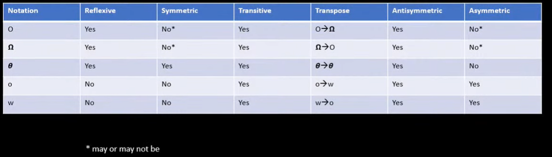
- Reflexive : \(f(n) = O(f(n)\) and \(f(n) = \Omega (f(n))\) and \(f(n) = \theta (f(n))\)
- Symmetric : If \(f(n) = \theta (g(n))\) then \(g(n) = \theta (f(n))\)
- Transitive : If \(f(n) = O(g(n))\) and \(g(n) = O(h(n))\) then \(f(n) = O(h(n))\)
- Transpose : If \(f(n) = O(g(n))\) then we can also conclude that \(g(n) = \Omega (f(n))\) so we say Big-Oh is transpose of Big-Omega and vice-versa.
- Antisymmetric : If \(f(n) = O(g(n))\) and \(g(n) = O(f(n))\) then we conclude that \(f(n) = g(n)\)
- Asymmetric : If \(f(n) = \omega (g(n))\) then we can conclude that \(g(n) \ne \omega (f(n))\)
3. Lecture 3
3.1. Calculating time complexity of algorithm
We will look at three types of situations
- Sequential instructions
- Iterative instructions
- Recursive instructions
3.1.1. Sequential instructions
A sequential set of instructions are instructions in a sequence without iterations and recursions. It is a simple block of instructions with no branches. A sequential set of instructions has time complexity of O(1), i.e., it has constant time complexity.
3.1.2. Iterative instructions
A set of instructions in a loop. Iterative instructions can have different complexities based on how many iterations occurs depending on input size.
- For fixed number of iterations (number of iterations known at compile time i.e. independant of the input size), the time complexity is constant, O(1). Example for(int i = 0; i < 100; i++) { … } will always have 100 iterations, so constant time complexity.
- For n number of iterations ( n is the input size ), the time complexity is O(n). Example, a loop for(int i = 0; i < n; i++){ … } will have n iterations where n is the input size, so complexity is O(n). Loop for(int i = 0; i < n/2; i++){…} also has time complexity O(n) because n/2 iterations are done by loop and 1/2 is constant thus not in big-oh notation.
- For a loop like for(int i = 1; i <= n; i = i*2){…} the value of i is update as *=2, so the number of iterations will be \(log_2 (n)\). Therefore, the time complexity is \(O(log_2 (n))\).
- For a loop like for(int i = n; i > 1; i = i/2){…} the value of i is update as *=2, so the number of iterations will be \(log_2 (n)\). Therefore, the time complexity is \(O(log_2 (n))\).
Nested Loops
- If inner loop iterator doesn't depend on outer loop, the complexity of the inner loop is multiplied by the number of times outer loop runs to get the time complexity For example, suppose we have loop as
for(int i = 0; i < n; i++){
  ...
  for(int j = 0; j < n; j *= 2){
    ...
  }
  ...
}
Here, the outer loop will n times and the inner loop will run log(n) times. Therefore, the total number of time statements in the inner loop run is n.log(n) times. Thus the time complexity is O(n.log(n)).
- If inner loop and outer loop are related, then complexities have to be computed using sums. Example, we have loop
for(int i = 0; i <= n; i++){
  ...
  for(int j = 0; j <= i; j++){
    ...
  }
  ...
}
Here the outer loop will run n times, so i goes from 0 to n. The number of times inner loop runs is j, which depends on i.
| Value of i | Number of times inner loop runs |
|---|---|
| 0 | 0 |
| 1 | 1 |
| 2 | 2 |
| . | . |
| . | . |
| . | . |
| n | n |
So the total number of times inner loop runs = \(1+2+3+....+n\)
total number of times inner loop runs = \(\frac{n.(n+1)}{2}\)
total number of times inner loop runs = \(\frac{n^2}{2} + \frac{n}{2}\)
Therefore, time complexity is \(O(\frac{n^2}{2} + \frac{n}{2}) = O(n^2)\)
Another example,
Suppose we have loop
for(int i = 1; i <= n; i++){
  ...
  for(int j = 1; j <= i; j *= 2){
    ...
  }
  ...
}
The outer loop will run n times with i from 1 to n, and inner will run log(i) times.
| Value of i | Number of times inner loop runs |
|---|---|
| 1 | log(1) |
| 2 | log(2) |
| 3 | log(3) |
| . | . |
| . | . |
| . | . |
| n | log(n) |
Thus, total number of times the inner loop runs is \(log(1) + log(2) + log(3) + ... + log(n)\).
total number of times inner loop runs = \(log(1.2.3...n)\)
total number of times inner loop runs = \(log(n!)\)
Using Stirling's approximation, we know that \(log(n!) = n.log(n) - n + 1\)
total number of times inner loop runs = \(n.log(n) - n + 1\)
Time complexity = \(O(n.log(n))\)
3.1.3. An example for time complexities of nested loops
Suppose a loop,
for(int i = 1; i <= n; i *= 2){
  ...
  for(int j = 1; j <= i; j *= 2){
    ...
  }
  ...
}
Here, outer loop will run log(n) times. Let's consider for some given n, it runs k times, i.e, let \[ k = log(n) \]
The inner loop will run log(i) times, so number of loops with changing values of i is
| Value of i | Number of times inner loop runs |
|---|---|
| 1 | log(1) |
| 21 | log(2) |
| 22 | 2.log(2) |
| 23 | 3.log(2) |
| . | . |
| . | . |
| . | . |
| 2k-1 | (k-1).log(2) |
So the total number of times inner loop runs is \(log(1) + log(2) + 2.log(2) + 3.log(2) + ... + (k-1).log(2)\) \[ \text{number of times inner loop runs} = log(1) + log(2).[1+2+3+...+(k-1)] \] \[ \text{number of times inner loop runs} = log(1) + log(2). \frac{(k-1).k}{2} \] \[ \text{number of times inner loop runs} = log(1) + log(2). \frac{k^2}{2} - \frac{k}{2} \] Putting value \(k = log(n)\) \[ \text{number of times inner loop runs} = log(1) + log(2). \frac{log^2(n)}{2} - \frac{log(n)}{2} \] \[ \text{Time complexity} = O(log^2(n)) \]
4. Lecture 4
4.1. Time complexity of recursive instructions
To get time complexity of recursive functions/calls, we first also show time complexity as recursive manner.
4.1.1. Time complexity in recursive form
We first have to create a way to describe time complexity of recursive functions in form of an equation as, \[ T(n) = ( \text{Recursive calls by the function} ) + ( \text{Time taken per call, i.e, the time taken except for recursive calls in the function} ) \]
- Example, suppose we have a recursive function
int fact(int n){
  if(n == 0 || n == 1)
    return 1;
  else
    return n * fact(n-1);
}
in this example, the recursive call is fact(n-1), therefore the time complexity of recursive call is T(n-1) and the time complexity of function except for recursive call is constant (let's assume c). So the time complexity is \[ T(n) = T(n-1) + c \] \[ T(1) = T(0) = C\ \text{where C is constant time} \]
- Another example,
int func(int n){
  if(n == 0 || n == 1)
    return 1;
  else
    return func(n - 1) * func(n - 2);
}
Here, the recursive calls are func(n-1) and func(n-2), therefore time complexities of recursive calls is T(n-1) and T(n-2). The time complexity of function except the recursive calls is constant (let's assume c), so the time complexity is \[ T(n) = T(n-1) + T(n-2) + c \] \[ T(1) = T(0) = C\ \text{where C is constant time} \]
- Another example,
int func(int n){
  int r = 0;
  for(int i = 0; i < n; i++)
    r += i;

  if(n == 0 || n == 1)
    return r;
  else
    return r * func(n - 1) * func(n - 2);
}
Here, the recursive calls are func(n-1) and func(n-2), therefore time complexities of recursive calls is T(n-1) and T(n-2). The time complexity of function except the recursive calls is θ (n) because of the for loop, so the time complexity is
\[ T(n) = T(n-1) + T(n-2) + n \] \[ T(1) = T(0) = C\ \text{where C is constant time} \]
4.2. Solving Recursive time complexities
4.2.1. Iterative method
- Take for example,
\[ T(1) = T(0) = C\ \text{where C is constant time} \] \[ T(n) = T(n-1) + c \]
We can expand T(n-1). \[ T(n) = [ T(n - 2) + c ] + c \] \[ T(n) = T(n-2) + 2.c \] Then we can expand T(n-2) \[ T(n) = [ T(n - 3) + c ] + 2.c \] \[ T(n) = T(n - 3) + 3.c \]
So, if we expand it k times, we will get
\[ T(n) = T(n - k) + k.c \] Since we know this recursion ends at T(1), let's put \(n-k=1\). Therefore, \(k = n-1\). \[ T(n) = T(1) + (n-1).c \]
Since T(1) = C \[ T(n) = C + (n-1).c \] So time complexity is, \[ T(n) = O(n) \]
- Another example,
\[ T(1) = C\ \text{where C is constant time} \] \[ T(n) = T(n-1) + n \]
Expanding T(n-1), \[ T(n) = [ T(n-2) + n - 1 ] + n \] \[ T(n) = T(n-2) + 2.n - 1 \]
Expanding T(n-2), \[ T(n) = [ T(n-3) + n - 2 ] + 2.n - 1 \] \[ T(n) = T(n-3) + 3.n - 1 - 2 \]
Expanding T(n-3), \[ T(n) = [ T(n-4) + n - 3 ] + 3.n - 1 - 2 \] \[ T(n) = T(n-4) + 4.n - 1 - 2 - 3 \]
So expanding till T(n-k) \[ T(n) = T(n-k) + k.n - [ 1 + 2 + 3 + .... + k ] \] \[ T(n) = T(n-k) + k.n - \frac{k.(k+1)}{2} \]
Putting \(n-k=1\). Therefore, \(k=n-1\). \[ T(n) = T(1) + (n-1).n - \frac{(n-1).(n)}{2} \] \[ T(n) = C + n^2 - n - \frac{n^2}{2} + \frac{n}{2} \]
Time complexity is \[ T(n) = O(n^2) \]
4.2.2. Master Theorem for Subtract recurrences
For recurrence relation of type
\[ T(n) = c\ for\ n \le 1 \] \[ T(n) = a.T(n-b) + f(n)\ for\ n > 1 \] \[ \text{where for f(n) we can say, } f(n) = O(n^k) \] \[ \text{where, a > 0, b > 0 and k} \ge 0 \]
- If a < 1, then T(n) = O(nk)
- If a = 1, then T(n) = O(nk+1)
- If a > 1, then T(n) = O(nk . an/b)
Example, \[ T(n) = 3T(n-1) + n^2 \]
Here, f(n) = O(n2), therfore k = 2,
Also, a = 3 and b = 1
Since a > 1, \(T(n) = O(n^2 . 3^n)\)
4.2.3. Master Theorem for divide and conquer recurrences
\[ T(n) = aT(n/b) + f(n).(log(n))^k \] \[ \text{here, f(n) is a polynomial function} \] \[ \text{and, a > 0, b > 0 and k } \ge 0 \] We calculate a value \(n^{log_ba}\)
- If \(\theta (f(n)) < \theta ( n^{log_ba} )\) then \(T(n) = \theta (n^{log_ba})\)
- If \(\theta (f(n)) > \theta ( n^{log_ba} )\) then \(T(n) = \theta (f(n).(log(n))^k )\)
- If \(\theta (f(n)) = \theta ( n^{log_ba} )\) then \(T(n) = \theta (f(n) . (log(n))^{k+1})\)
For the above comparision, we say higher growth rate is greater than slower growth rate. Eg, θ (n2) > θ (n).
Example, calculating complexity for
\[ T(n) = T(n/2) + 1 \]
Here, f(n) = 1
Also, a = 1, b = 2 and k = 0.
Calculating nlogba = nlog21 = n0 = 1
Therfore, θ (f(n)) = θ (nlogba)
So time complexity is
\[ T(n) = \theta ( 1 . (log(n))^{0 + 1} ) \]
\[ T(n) = \theta (log(n)) \]
Another example, calculate complexity for \[ T(n) = 2T(n/2) + nlog(n) \]
Here, f(n) = n
Also, a = 2, b = 2 and k = 1
Calculating nlogba = nlog22 = n
Therefore, θ (f(n)) = θ (nlogba)
So time complexity is,
\[ T(n) = \theta ( n . (log(n))^{2}) \]
4.3. Square root recurrence relations
4.3.1. Iterative method
Example, \[ T(n) = T( \sqrt{n} ) + 1 \] we can write this as, \[ T(n) = T( n^{1/2}) + 1 \] Now, we expand \(T( n^{1/2})\) \[ T(n) = [ T(n^{1/4}) + 1 ] + 1 \] \[ T(n) = T(n^{1/(2^2)}) + 1 + 1 \] Expand, \(T(n^{1/4})\) \[ T(n) = [ T(n^{1/8}) + 1 ] + 1 + 1 \] \[ T(n) = T(n^{1/(2^3)}) + 1 + 1 + 1 \]
Expanding k times, \[ T(n) = T(n^{1/(2^k)}) + 1 + 1 ... \text{k times } + 1 \] \[ T(n) = T(n^{1/(2^k)}) + k \]
Let's consider \(T(2)=C\) where C is constant.
Putting \(n^{1/(2^k)} = 2\)
\[ \frac{1}{2^k} log(n) = log(2) \]
\[ \frac{1}{2^k} = \frac{log(2)}{log(n)} \]
\[ 2^k = \frac{log(n)}{log(2)} \]
\[ 2^k = log_2n \]
\[ k = log(log(n)) \]
So putting k in time complexity equation, \[ T(n) = T(2) + log(log(n)) \] \[ T(n) = C + log(log(n)) \] Time complexity is, \[ T(n) = \theta (log(log(n))) \]
4.3.2. Master Theorem for square root recurrence relations
For recurrence relations with square root, we need to first convert the recurrance relation to the form with which we use master theorem. Example, \[ T(n) = T( \sqrt{n} ) + 1 \] Here, we need to convert \(T( \sqrt{n} )\) , we can do that by substituting \[ \text{Substitute } n = 2^m \] \[ T(2^m) = T ( \sqrt{2^m} ) + 1 \] \[ T(2^m) = T ( 2^{m/2} ) + 1 \]
Now, we need to consider a new function such that,
\[ \text{Let, } S(m) = T(2^m) \]
Thus our time recurrance relation will become,
\[ S(m) = S(m/2) + 1 \]
Now, we can apply the master's theorem.
Here, f(m) = 1
Also, a = 1, and b = 2 and k = 0
Calculating mlogba = mlog21 = m0 = 1
Therefore, θ (f(m)) = θ ( mlogba )
So by master's theorem,
\[ S(m) = \theta (1. (log(m))^{0+1} ) \]
\[ S(m) = \theta (log(m) ) \]
Now, putting back \(m = log(n)\)
\[ T(n) = \theta (log(log(n))) \]
Another example,
\[ T(n) = 2.T(\sqrt{n})+log(n) \]
Substituting \(n = 2^m\)
\[ T(2^m) = 2.T(\sqrt{2^m}) + log(2^m) \]
\[ T(2^m) = 2.T(2^{m/2}) + m \]
Consider a function \(S(m) = T(2^m)\)
\[ S(m) = 2.S(m/2) + m \]
Here, f(m) = m
Also, a = 2, b = 2 and k = 0
Calculating mlogba = mlog22 = 1
Therefore, θ (f(m)) > θ (mlogba)
Using master's theorem,
\[ S(m) = \theta (m.(log(m))^0 ) \]
\[ S(m) = \theta (m.1) \]
Putting value of m,
\[ T(n) = \theta (log(n)) \]
5. Lecture 5
5.1. Extended Master's theorem for time complexity of recursive algorithms
5.1.1. For (k = -1)
\[ T(n) = aT(n/b) + f(n).(log(n))^{-1} \] \[ \text{Here, } f(n) \text{ is a polynomial function} \] \[ a > 0\ and\ b > 1 \]
- If θ (f(n)) < θ ( nlogba ) then, T(n) = θ (nlogba)
- If θ (f(n)) > θ ( nlogba ) then, T(n) = θ (f(n))
- If θ (f(n)) < θ ( nlogba ) then, T(n) = θ (f(n).log(log(n)))
5.1.2. For (k < -1)
\[ T(n) = aT(n/b) + f(n).(log(n))^{k} \] \[ \text{Here, } f(n) \text{ is a polynomial function} \] \[ a > 0\ and\ b > 1\ and\ k < -1 \]
- If θ (f(n)) < θ ( nlogba ) then, T(n) = θ (nlogba)
- If θ (f(n)) > θ ( nlogba ) then, T(n) = θ (f(n))
- If θ (f(n)) < θ ( nlogba ) then, T(n) = θ (nlogba)
5.2. Tree method for time complexity of recursive algorithms
Tree method is used when there are multiple recursive calls in our recurrance relation. Example, \[ T(n) = T(n/5) + T(4n/5) + f(n) \] Here, one call is T(n/5) and another is T(4n/5). So we can't apply master's theorem. So we create a tree of recursive calls which is used to calculate time complexity. The first node, i.e the root node is T(n) and the tree is formed by the child nodes being the calls made by the parent nodes. Example, let's consider the recurrance relation \[ T(n) = T(n/5) + T(4n/5) + f(n) \]
      +-----T(n/5)
T(n)--+
      +-----T(4n/5)
Since T(n) calls T(n/5) and T(4n/5), the graph for that is shown as drawn above. Now using recurrance relation, we can say that T(n/5) will call T(n/52) and T(4n/52). Also, T(4n/5) will call T(4n/52) and T(42 n/ 52).
		    +--T(n/5^2)
      +-----T(n/5)--+
      +             +--T(4n/5^2)
T(n)--+
      +             +--T(4n/5^2)
      +-----T(4n/5)-+
		    +--T(4^2 n/5^2)
Suppose we draw this graph for an unknown number of levels.
		    +--T(n/5^2)- - - - - - -  etc.
      +-----T(n/5)--+
      +             +--T(4n/5^2) - - - - - - - - - etc.
T(n)--+
      +             +--T(4n/5^2) - - - - - -  - - - etc.
      +-----T(4n/5)-+
		    +--T(4^2 n/5^2)- - - - - - etc.
We will now replace T()'s with the cost of the call. The cost of the call is f(n), i.e, the time taken other than that caused by the recursive calls.
		    +--f(n/5^2)- - - - - - -  etc.
      +-----f(n/5)--+
      +             +--f(4n/5^2) - - - - - - - - - etc.
f(n)--+
      +             +--f(4n/5^2) - - - - - -  - - - etc.
      +-----f(4n/5)-+
		    +--f(4^2 n/5^2)- - - - - - etc.
In our example, let's assume f(n) = n, therfore,
		  +--  n/5^2 - - - - - - -  etc.
    +-----  n/5 --+
    +             +-- 4n/5^2  - - - - - - - - - etc.
n --+
    +             +--  4n/5^2  - - - - - -  - - -etc.
    +-----  4n/5 -+
		  +--  4^2 n/5^2 - - - - - -  etc.
Now we can get cost of each level.
			   +--  n/5^2 - - - - - - -  etc.
	     +-----  n/5 --+
	     +             +-- 4n/5^2  - - - - - - - - - etc.
	 n --+
	     +             +--  4n/5^2  - - - - - -  - - -etc.
	     +----- 4n/5 --+
			   +--  4^2 n/5^2 - - - - - -  etc.


Sum :    n         n/5         n/25
		  +4n/5       +4n/25
			      +4n/25
			      +16n/25
       .....      .....       ......
	 n          n           n
Since sum on all levels is n, we can say that Total time taken is \[ T(n) = \Sigma \ (cost\ of\ level_i) \]
Now we need to find the longest branch in the tree. If we follow the pattern of expanding tree in a sequence as shown, then the longest branch is always on one of the extreme ends of the tree. So for our example, if tree has (k+1) levels, then our branch is either (n/5k) of (4k n/5k). Consider the terminating condition is, \(T(a) = C\). Then we will calculate value of k by equating the longest branch as, \[ \frac{n}{5^k} = a \] \[ k = log_5 (n/a) \] Also, \[ \frac{4^k n}{5^k} = a \] \[ k = log_{5/4} n/a \]
So, we have two possible values of k, \[ k = log_{5/4}(n/a),\ log_5 (n/a) \]
Now, we can say that, \[ T(n) = \sum_{i=1}^{k+1} \ (cost\ of\ level_i) \] Since in our example, cost of every level is n. \[ T(n) = n.(k+1) \] Putting values of k, \[ T(n) = n.(log_{5/4}(n/a) + 1) \] or \[ T(n) = n.(log_{5}(n/a) + 1) \]
Of the two possible time complexities, we consider the one with higher growth rate in the big-oh notation.
5.2.1. Avoiding tree method
The tree method as mentioned is mainly used when we have multiple recursive calls with different factors. But when using the big-oh notation (O). We can avoid tree method in favour of the master's theorem by converting recursive call with smaller factor to larger. This works since big-oh calculates worst case. Let's take our previous example \[ T(n) = T(n/5) + T(4n/5) + f(n) \] Since T(n) is an increasing function. We can say that \[ T(n/5) < T(4n/5) \] So we can replace smaller one and approximate our equation to, \[ T(n) = T(4n/5) + T(4n/5) + f(n) \] \[ T(n) = 2.T(4n/5) + f(n) \]
Now, our recurrance relation is in a form where we can apply the mater's theorem.
5.3. Space complexity
The amount of memory used by the algorithm to execute and produce the result for a given input size is space complexity. Similar to time complexity, when comparing two algorithms space complexity is usually represented as the growth rate of memory used with respect to input size. The space complexity includes
- Input space : The amount of memory used by the inputs to the algorithm.
- Auxiliary space : The amount of memory used during the execution of the algorithm, excluding the input space.
NOTE : Space complexity by definition includes both input space and auxiliary space, but when comparing algorithms the input space is often ignored. This is because two algorithms that solve the same problem will have same input space based on input size (Example, when comparing two sorting algorithms, the input space will be same because both get a list as an input). So from this point on, refering to space complexity, we are actually talking about Auxiliary Space Complexity, which is space complexity but only considering the auxiliary space.
5.3.1. Auxiliary space complexity
The space complexity when we disregard the input space is the auxiliary space complexity, so we basically treat algorithm as if it's input space is zero. Auxiliary space complexity is more useful when comparing algorithms because the algorithms which are working towards same result will have the same input space, Example, the sorting algorithms will all have the input space of the list, so it is not a metric we can use to compare algorithms. So from here, when we calculate space complexity, we are trying to calculate auxiliary space complexity and sometimes just refer to it as space complexity.
5.4. Calculating auxiliary space complexity
There are two parameters that affect space complexity,
- Data space : The memory taken by the variables in the algorithm. So allocating new memory during runtime of the algorithm is what forms the data space. The space which was allocated for the input space is not considered a part of the data space.
- Code Execution Space : The memory taken by the instructions themselves is called code execution space. Unless we have recursion, the code execution space remains constant since the instructions don't change during runtime of the algorithm. When using recursion, the instructions are loaded again and again in memory, thus increasing code execution space.
5.4.1. Data Space used
The data space used by the algorithm depends on what data structures it uses to solve the problem. Example,
/* Input size of n */
void algorithms(int n){
  /* Creating an array of whose size depends on input size */
  int data[n];

  for(int i = 0; i < n; i++){
    int x = data[i];
    // Work on data
  }
}
Here, we create an array of size n, so the increase in allocated space increases with the input size. So the space complexity is, \(\theta (n)\).
- Another example,
/* Input size of n */
void algorithms(int n){
  /* Creating a matrix sized n*n of whose size depends on input size */
  int data[n][n];

  for(int i = 0; i < n; i++){
    for(int j = 0; j < n; j++){
      int x = data[i][j];
      // Work on data
    }
  }
}
Here, we create a matrix of size n*n, so the increase in allocated space increases with the input size by \(n^2\). So the space complexity is, \(\theta (n^2)\).
- If we use a node based data structure like linked list or trees, then we can show space complexity as the number of nodes used by algorithm based on input size, (if all nodes are of equal size).
- Space complexity of the hash map is considered O(n) where n is the number of entries in the hash map.
5.4.2. Code Execution space in recursive algorithm
When we use recursion, the function calls are stored in the stack. This means that code execution space will increase. A single function call has fixed (constant) space it takes in the memory. So to get space complexity, we need to know how many function calls occur in the longest branch of the function call tree.
- NOTE : Space complexity only depends on the longest branch of the function calls tree.
- The tree is made the same way we make it in the tree method for calculating time complexity of recursive algorithms
This is because at any given time, the stack will store only a single branch.
- Example,
int func(int n){
  if(n == 1 || n == 0)
    return 1;
  else
    return n * func(n - 1);
}
To calculate space complexity we can use the tree method. But rather than when calculating time complexity, we will count the number of function calls using the tree.
We will do this by drawing tree of what function calls will look like for given input size n.
The tree for k+1 levels is,
func(n)--func(n-1)--func(n-2)--.....--func(n-k)
This tree only has a single branch. To get the number of levels for a branch, we put the terminating condition at the extreme branches of the tree. Here, the terminating condition is func(1), therefore, we will put \(func(1) = func(n-k)\), i.e, \[ 1 = n - k \] \[ k + 1 = n \]
So the number of levels is \(n\). Therefore, space complexity is \(\theta (n)\)
- Another example,
void func(int n){
  if(n/2 <= 1)
    return n;
  func(n/2);
  func(n/2);
}
Drawing the tree for k+1 levels.
			  +--func(n/2^2)- - - - - - -  func(n/2^k)
	 +-----func(n/2)--+
	 +                +--func(n/2^2) - - - - - - - - - func(n/2^k)
func(n)--+
	 +               +--func(n/2^2) - - - - - -  - - - func(n/2^k)
	 +-----func(n/2)-+
			 +--func(n/2^2)- - - - - - func(n/2^k)
- As we know from the tree method, the two extreme branches of the tree will always be the longest ones.
Both the extreme branches have the same call which here is func(n/2k). To get the number of levels for a branch, we put the terminating condition at the extreme branches of the tree. Here, the terminating condition is func(2), therefore, we will put \(func(2) = func(n/2^k)\), i.e, \[ 2 = \frac{n}{2^k} \] \[ k + 1 = log_2n \] Number of levels is \(log_2n\). Therefore, space complexity is \(\theta (log_2n)\).
6. Lecture 6
6.1. Divide and Conquer algorithms
Divide and conquer is a problem solving strategy. In divide and conquer algorithms, we solve problem recursively applying three steps :
- Divide : Problem is divided into smaller problems that are instances of same problem.
- Conquer : If subproblems are large, divide and solve them recursivly. If subproblem is small enough then solve it in a straightforward method
- Combine : combine the solutions of subproblems into the solution for the original problem.
Example,
- Binary search
- Quick sort
- Merge sort
- Strassen's matrix multiplication
6.2. Searching for element in array
6.2.1. Straight forward approach for searching (Linear Search)
int linear_search(int *array, int n, int x){
  for(int i = 0; i < n; i++){
    if(array[i] == x){
      printf("Found at index : %d", i);
      return i;
    }
  }
  return -1;
}
Recursive approach
// call this function with index = 0
int linear_search(int array[], int item, int index){
  if( index >= len(array) )
    return -1;
  else if (array[index] == item)
    return index;
  else
    return linear_search(array, item, index + 1);
}
Recursive time complexity : \(T(n) = T(n-1) + 1\)
- Best Case : The element to search is the first element of the array. So we need to do a single comparision. Therefore, time complexity will be constant O(1).
- Worst Case : The element to search is the last element of the array. So we need to do n comparisions for the array of size n. Therefore, time complexity is O(n).
- Average Case : For calculating the average case, we need to consider the average number of comparisions done over all possible cases.
| Position of element to search (x) | Number of comparisions done |
|---|---|
| 0 | 1 |
| 1 | 2 |
| 2 | 3 |
| . | . |
| . | . |
| . | . |
| n-1 | n |
| ……………….. | ……………….. |
| Sum | \(\frac{n(n+1)}{2}\) |
\[ \text{Average number of comparisions} = \frac{ \text{Sum of number of comparisions of all cases} }{ \text{Total number of cases.} } \] \[ \text{Average number of comparisions} = \frac{n(n+1)}{2} \div n \] \[ \text{Average number of comparisions} = \frac{n+1}{2} \] \[ \text{Time complexity in average case} = O(n) \]
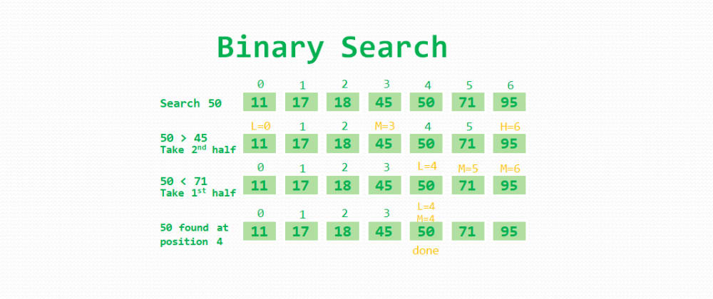
6.2.2. Divide and conquer approach (Binary search)
The binary search algorithm works on an array which is sorted. In this algorithm we:
- Check the middle element of the array, return the index if element found.
- If element > array[mid], then our element is in the right part of the array, else it is in the left part of the array.
- Get the mid element of the left/right sub-array
- Repeat this process of division to subarray's and comparing the middle element till our required element is found.
The divide and conquer algorithm works as,
Suppose binarySearch(array, left, right, key), left and right are indicies of left and right of subarray. key is the element we have to search.
- Divide part : calculate mid index as mid = left + (right - left) /2 or (left + right) / 2. If array[mid] == key, return the value of mid.
- Conquer part : if array[mid] > key, then key must not be in right half. So we search for key in left half, so we will recursively call binarySearch(array, left, mid - 1, key). Similarly, if array[mid] < key, then key must not be in left half. So we search for key in right half, so recursively call binarySearch(array, mid + 1, right, key).
- Combine part : Since the binarySearch function will either return -1 or the index of the key, there is no need to combine the solutions of the subproblems.
int binary_search(int *array, int n, int x){
  int low = 0;
  int high = n;

  int mid = (low + high) / 2;

  while(low <= high){
    mid = (low + high) / 2;
    if (x == array[mid]){
      return mid;
    }else if (x < array[mid]){
      low = low;
      high = mid - 1;
    }else{
      low = mid + 1;
      high = high;
    }
  }

  return -1;
}
Recursive approach:
int binary_search(int *array, int left, int right, int x){
  if(left > right)
    return -1;

  int mid = (left + right) / 2;
  // or we can use mid = left + (right - left) / 2, this will avoid int overflow when array has more elements.

  if (x == array[mid])
    return mid;
  else if (x < array[mid])
    return binary_search(array, left, mid - 1, x);
  else
    return binary_search(array, mid + 1, right, x);
}
Recursive time complexity : \(T(n) = T(n/2) + 1\)
- Best Case : Time complexity = O(1)
- Average Case : Time complexity = O(log n)
- Worst Case : Time complexity = O(log n)
Binary search is better for sorted arrays and linear search is better for sorted arrays.
Another way to visualize binary search is using the binary tree.
6.3. Max and Min element from array
6.3.1. Straightforward approach
struc min_max {int min; int max;}
min_max(int array[]){
  int max = array[0];
  int min = array[0];

  for(int i = 0; i < len(array); i++){
    if(array[i] > max)
      max = array[i];
    else if(array[i] < min)
      min = array[i];
  }

  return (struct min_max) {min, max};
}
- Best case : array is sorted in ascending order. Number of comparisions is \(n-1\). Time complexity is \(O(n)\).
- Worst case : array is sorted in descending order. Number of comparisions is \(2.(n-1)\). Time complexity is \(O(n)\).
- Average case : array can we arranged in n! ways, this makes calculating number of comparisions in the average case hard and it is somewhat unnecessary, so it is skiped. Time complexity is \(O(n)\)
6.3.2. Divide and conquer approach
Suppose the function is MinMax(array, left, right) which will return a tuple (min, max). We will divide the array in the middle, mid = (left + right) / 2. The left array will be array[left:mid] and right aray will be array[mid+1:right]
- Divide part : Divide the array into left array and right array. If array has only single element then both min and max are that single element, if array has two elements then compare the two and the bigger element is max and other is min.
- Conquer part : Recursively get the min and max of left and right array, leftMinMax = MinMax(array, left, mid) and rightMinMax = MinMax(array, mid + 1, right).
- Combine part : If leftMinMax[0] > rightMinmax[0], then min = righMinMax[0], else min = leftMinMax[0]. Similarly, if leftMinMax[1] > rightMinMax[1], then max = leftMinMax[1], else max = rightMinMax[1].
# Will return (min, max)
def minmax(array, left, right):
    if left == right:       # Single element in array
        return (array[left], array[left])
    elif left + 1 == right: # Two elements in array
        if array[left] > array[right]:
            return (array[right], array[left])
        else:
            return (array[left], array[right])
    else:                  # More than two elements
        mid = (left + right) / 2
        minimum, maximum = 0, 0
        leftMinMax = minmax(array, left, mid)
        rightMinMax = minmax(array, mid + 1, right)

        # Combining result of the minimum from left and right subarray's
        if leftMinMax[0] > rightMinMax[0]:
            minimum = rightMinMax[0]
        else:
            minimum = leftMinMax[0]

        # Combining result of the maximum from left and right subarray's
        if leftMinMax[1] > rightMinMax[1]:
            maximum = leftMinMax[1]
        else:
            maximum = rightMinMax[1]

        return (minimum, maximum)
- Time complexity
We are dividing the problem into two parts of approximately, and it takes two comparisions on each part. Let's consider a comparision takes unit time. Then time complexity is
\[ T(n) = T(n/2) + T(n/2) + 2 \]
\[ T(n) = 2.T(n/2) + 2 \]
The recurrance terminated if single element in array with zero comparisions, i.e, \(T(1) = 0\), or when two elements with single comparision \(T(2) = 1\).
Now we can use the master's theorem or tree method to solve for time complexity.
\[ T(n) = \theta (n) \]
- Space complexity
For space complexity, we need to find the longest branch of the recursion tree. Since both recursive calls are same sized, and the factor is (1/2), for k+1 levels, function call will be func(n/2k), and terminating condition is func(2) \[ func(2) = func(n/2^k) \] \[ 2 = \frac{n}{2^k} \] \[ k + 1 = log_2n \] Since longest branch has \(log_2n\) nodes, the space complexity is \(O(log_2n)\).
- Number of comparisions
In every case i.e, average, best and worst cases, the number of comparisions in this algorithm is same. \[ \text{Total number of comparisions} = \frac{3n}{2} - 2 \] If n is not a power of 2, we will round the number of comparision up.
6.3.3. Efficient single loop approach (Increment by 2)
In this algorithm we will compare pairs of numbers from the array. It works on the idea that the larger number of the two in pair can be the maximum number and smaller one can be the minimum one. So after comparing the pair, we can simply test from maximum from the bigger of two an minimum from smaller of two. This brings number of comparisions to check two numbers in array from 4 (when we increment by 1) to 3 (when we increment by 2).
def min_max(array):
    (minimum, maximum) = (array[0], array[0])
    i = 1
    while i < len(array):
        if i + 1 == len(array):  # don't check i+1, it's out of bounds, break the loop after checking a[i]
            if array[i] > maximum:
                maximum = array[i]
            elif array[i] < minimum:
                minimum = array[i]
            break

        if array[i] > array[i + 1]:
            # check possibility that array[i] is maximum and array[i+1] is minimum
            if array[i] > maximum:
                maximum = array[i]
            if array[i + 1] < minimum:
                minimum = array[i + 1]
        else:
            # check possibility that array[i+1] is maximum and array[i] is minimum
            if array[i + 1] > maximum:
                maximum = array[i + 1]
            if array[i] < minimum:
                minimum = array[i]

        i += 2
    return (minimum, maximum)
- Time complexity = O(n)
- Space complexity = O(1)
- Total number of comparisions = \[ \text{If n is odd}, \frac{3(n-1)}{2} \] \[ \text{If n is even}, \frac{3n}{2} - 2 \]
7. Lecture 7
7.1. Square matrix multiplication
Matrix multiplication algorithms taken from here: https://www.cs.mcgill.ca/~pnguyen/251F09/matrix-mult.pdf
7.1.1. Straight forward method
/* This will calculate A X B and store it in C. */
#define N 3

int main(){
  int A[N][N] = {
    {1,2,3},
    {4,5,6},
    {7,8,9} };

  int B[N][N] = {
    {10,20,30},
    {40,50,60},
    {70,80,90} };

  int C[N][N];

  for(int i = 0; i < N; i++){
    for(int j = 0; j < N; j++){
      C[i][j] = 0;
      for(int k = 0; k < N; k++){
        C[i][j] += A[i][k] * B[k][j];
      }
    }
  }

  return 0;
}
Time complexity is \(O(n^3)\)
7.1.2. Divide and conquer approach
The divide and conquer algorithm only works for a square matrix whose size is n X n, where n is a power of 2. The algorithm works as follows.
MatrixMul(A, B, n):
  If n == 2 {
    return A X B
  }else{
    Break A into four parts A_11, A_12, A_21, A_22, where A = [[ A_11, A_12],
							       [ A_21, A_22]]

    Break B into four parts B_11, B_12, B_21, B_22, where B = [[ B_11, B_12],
							       [ B_21, B_22]]

    C_11 = MatrixMul(A_11, B_11, n/2) + MatrixMul(A_12, B_21, n/2)
    C_12 = MatrixMul(A_11, B_12, n/2) + MatrixMul(A_12, B_22, n/2)
    C_21 = MatrixMul(A_21, B_11, n/2) + MatrixMul(A_22, B_21, n/2)
    C_22 = MatrixMul(A_21, B_12, n/2) + MatrixMul(A_22, B_22, n/2)

    C = [[ C_11, C_12],
	 [ C_21, C_22]]

    return C
  }
The addition of matricies of size (n X n) takes time \(\theta (n^2)\), therefore, for computation of C11 will take time of \(\theta \left( \left( \frac{n}{2} \right)^2 \right)\), which is equals to \(\theta \left( \frac{n^2}{4} \right)\). Therefore, computation time of C11, C12, C21 and C22 combined will be \(\theta \left( 4 \frac{n^2}{4} \right)\), which is equals to \(\theta (n^2)\).
There are 8 recursive calls in this function with MatrixMul(n/2), therefore, time complexity will be
\[ T(n) = 8T(n/2) + \theta (n^2) \]
Using the master's theorem
\[ T(n) = \theta (n^{log_28}) \]
\[ T(n) = \theta (n^3) \]
7.1.3. Strassen's algorithm
Another, more efficient divide and conquer algorithm for matrix multiplication. This algorithm also only works on square matrices with n being a power of 2. This algorithm is based on the observation that, for A X B = C. We can calculate C11, C12, C21 and C22 as,
\[ \text{C_11 = P_5 + P_4 - P_2 + P_6} \] \[ \text{C_12 = P_1 + P_2} \] \[ \text{C_21 = P_3 + P_4} \] \[ \text{C_22 = P_1 + P _5 - P_3 - P_7} \] Where, \[ \text{P_1 = A_11 X (B_12 - B_22)} \] \[ \text{P_2 = (A_11 + A_12) X B_22} \] \[ \text{P_3 = (A_21 + A_22) X B_11} \] \[ \text{P_4 = A_22 X (B_21 - B_11)} \] \[ \text{P_5 = (A_11 + A_22) X (B_11 + B_22)} \] \[ \text{P_6 = (A_12 - A_22) X (B_21 + B_22)} \] \[ \text{P_7 = (A_11 - A_21) X (B_11 + B_12)} \] This reduces number of recursion calls from 8 to 7.
Strassen(A, B, n):
  If n == 2 {
    return A X B
  }
  Else{
    Break A into four parts A_11, A_12, A_21, A_22, where A = [[ A_11, A_12],
							       [ A_21, A_22]]

    Break B into four parts B_11, B_12, B_21, B_22, where B = [[ B_11, B_12],
							       [ B_21, B_22]]
    P_1 = Strassen(A_11, B_12 - B_22, n/2)
    P_2 = Strassen(A_11 + A_12, B_22, n/2)
    P_3 = Strassen(A_21 + A_22, B_11, n/2)
    P_4 = Strassen(A_22, B_21 - B_11, n/2)
    P_5 = Strassen(A_11 + A_22, B_11 + B_22, n/2)
    P_6 = Strassen(A_12 - A_22, B_21 + B_22, n/2)
    P_7 = Strassen(A_11 - A_21, B_11 + B_12, n/2)
    C_11 = P_5 + P_4 - P_2 + P_6
    C_12 = P_1 + P_2
    C_21 = P_3 + P_4
    C_22 = P_1 + P_5 - P_3 - P_7
    C = [[ C_11, C_12],
	 [ C_21, C_22]]
    return C
  }
This algorithm uses 18 matrix addition operations. So our computation time for that is \(\theta \left(18\left( \frac{n}{2} \right)^2 \right)\) which is equal to \(\theta (4.5 n^2)\) which is equal to \(\theta (n^2)\).
There are 7 recursive calls in this function which are Strassen(n/2), therefore, time complexity is
\[ T(n) = 7T(n/2) + \theta (n^2) \]
Using the master's theorem
\[ T(n) = \theta (n^{log_27}) \]
\[ T(n) = \theta (n^{2.807}) \]
- NOTE : The divide and conquer approach and strassen's algorithm typically use n == 1 as their terminating condition since for multipliying 1 X 1 matrices, we only need to calculate product of the single element they contain, that product is thus the single element of our resultant 1 X 1 matrix.
7.2. Sorting algorithms
7.2.1. In place vs out place sorting algorithm
If the space complexity of a sorting algorithm is \(\theta (1)\), then the algorithm is called in place sorting, else the algorithm is called out place sorting.
7.2.2. Bubble sort
Simplest sorting algorithm, easy to implement so it is useful when number of elements to sort is small. It is an in place sorting algorithm. We will compare pairs of elements from array and swap them to be in correct order. Suppose input has n elements.
- For first pass of the array, we will do n-1 comparisions between pairs, so 1st and 2nd element; then 2nd and 3rd element; then 3rd and 4th element; till comparision between (n-1)th and nth element, swapping positions according to the size. A single pass will put a single element at the end of the list at it's correct position.
- For second pass of the array, we will do n-2 comparisions because the last element is already in it's place after the first pass.
- Similarly, we will continue till we only do a single comparision.
- The total number of comparisions will be \[ \text{Total comparisions} = (n - 1) + (n - 2) + (n - 3) + ..... + 2 + 1 \] \[ \text{Total comparisions} = \frac{n(n-1)}{2} \] Therefore, time complexity is \(\theta (n^2)\)
void binary_search(int array[]){
  /* i is the number of comparisions in the pass */
  for(int i = len(array) - 1; i >= 1; i--){
    /* j is used to traverse the list */
    for(int j = 0; j < i; j++){
      if(array[j] > array[j+1])
        array[j], array[j+1] = array[j+1], array[j];
    }
  }
}
Minimum number of swaps can be calculated by checking how many swap operations are needed to get each element in it's correct position. This can be done by checking the number of smaller elements towards the left. For descending, check the number of larger elements towards the left of the given element. Example for ascending sort,
| Array | 21 | 16 | 17 | 8 | 31 |
| Minimum number of swaps to get in correct position | 3 | 1 | 0 | 0 | 0 |
Therefore, minimum number of swaps is ( 3 + 1 + 0 + 0 + 0) , which is equal to 4 swaps.
- Reducing number of comparisions in implementation : at the end of every pass, check the number of swaps. If number of swaps in a pass is zero, then the array is sorted. This implementation does not give minimum number of comparisions, but reduces number of comparisions from default implementation. It reduces the time complexity to \(\theta (n)\) for best case scenario, since we only need to pass through array once.
Recursive time complexity : \(T(n) = T(n-1) + n - 1\)
8. Lecture 8
8.1. Selection sort
It is an inplace sorting technique. In this algorithm, we will get the minimum element from the array, then we swap it to the first position. Now we will get the minimum from array[1:] and place it in index 1. Similarly, we get minimum from array[2:] and then place it on index 2. We do till we get minimum from array[len(array) - 2:] and place minimum on index [len(array) - 2].
void selection_sort(int array[]){
  for( int i = 0; i < len(array)-2 ; i++ ) {
    /* Get the minimum index from the sub-array [i:] */
    int min_index = i;
    for( int j = i+1; j < len(array) - 1; j++ )
      if (array[j] < array[min_index]) { min_index = j; }

    /* Swap the min_index with it's position at start of sub-array */
    array[i], array[min_index] = array[min_index], array[i];
  }
}
8.1.1. Time complexity
The total number of comparisions is, \[ \text{Total number of comparisions} = (n -1) + (n-2) + (n-3) + ... + (1) \] \[ \text{Total number of comparisions} = \frac{n(n-1)}{2} \] For this algorithm, number of comparisions are same in best, average and worst case. Therefore the time complexity in all cases is, \[ \text{Time complexity} = \theta (n) \]
- Recurrance time complexity : \(T(n) = T(n-1) + n - 1\)
8.2. Insertion sort
It is an inplace sorting algorithm.
- In this algorithm, we first divide array into two sections. Initially, the left section has a single element and right section has all the other elements. Therefore, the left part is sorted and right part is unsorted.
- We call the leftmost element of the right section the key.
- Now, we insert the key in it's correct position, in left section.
- As commanly known, for insertion operation we need to shift elements. So we shift elements in the left section.
void insertion_sort ( int array[] ) {
  for( int i = 1; i < len(array); i++ ) {
    /* Key is the first element of the right section of array */
    int key = array[j];
    int j = i - 1;

    /* Shift till we find the correct position of the key in the left section */
    while ( j > 0 && array[j] > key ) {
      array[j + 1] = array[j];
      j -= 1;
    }
    /* Insert key in it's correct position */
    array[j+1] = key;
  }
}
8.2.1. Time complexity
Best Case : The best case is when input array is already sorted. In this case, we do (n-1) comparisions and no swaps. The time complexity will be \(\theta (n)\)
Worst Case : The worst case is when input array is is descending order when we need to sort in ascending order and vice versa (basically reverse of sorted). The number of comparisions is
\[ [1 + 2 + 3 + .. + (n-1)] = \frac{n(n-1)}{2} \]
The number of element shift operations is
\[ [1 + 2 + 3 + .. + (n-1)] = \frac{n(n-1)}{2} \]
Total time complexity becomes \(\theta \left( 2 \frac{n(n-1)}{2} \right)\), which is simplified to \(\theta (n^2)\).
- NOTE : Rather than using linear search to find the position of key in the left (sorted) section, we can use binary search to reduce number of comparisions.
8.3. Inversion in array
The inversion of array is the measure of how close array is from being sorted.
For an ascending sort, it is the amount of element pairs such that array[i] > array[j] and i < j OR IN OTHER WORDS array[i] < array[j] and i > j.
- For ascending sort, we can simply look at the number of elements to left of the given element that are smaller.
| Array | 10 | 6 | 12 | 8 | 3 | 1 |
| Inversions | 4 | 2 | 3 | 2 | 1 | 0 |
Total number of inversions = (4+2+3+2+1+0) = 12
- For descending sort, we can simply look at the number of elements to the left of the given element that are larger.
| Array | 10 | 6 | 12 | 8 | 3 | 1 |
| Inversions | 1 | 2 | 0 | 0 | 0 | 0 |
Total number of inversions = 1 + 2 = 3
- For an array of size n
\[ \text{Maximum possible number of inversions} = \frac{n(n-1)}{2} \] \[ \text{Minimum possible number of inversions} = 0 \]
8.3.1. Relation between time complexity of insertion sort and inversion
If the inversion of an array is f(n), then the time complexity of the insertion sort will be \(\theta (n + f(n))\).
8.4. Quick sort
It is a divide and conquer technique. It uses a partition algorithm which will choose an element from array, then place all smaller elements to it's left and larger to it's right. Then we can take these two parts of the array and recursively place all elements in correct position. For ease, the element chosen by the partition algorithm is either leftmost or rightmost element.
void quick_sort(int array[], int low, int high){
  if(low < high){
    int x = partition(array, low, high);
    quick_sort(array, low, x-1);
    quick_sort(array, x+1, high);
  }
}
As we can see, the main component of this algorithm is the partition algorithm.
8.4.1. Lomuto partition
The partition algorithm will work as follows:
/* Will return the index where the array is partitioned */
int partition(int array[], int low, int high){
  int pivot = array[high];
  /* This will point to the element greater than pivot */
  int i = low - 1;

  for(int j = low; j < high; j++){
    if(array[j] <= pivot){
      i += 1;
      array[i], array[j] = array[j], array[i];
    }
  }

  array[i+1], array[high] = array[high], array[i+1];
  return (i + 1);
}
- Time complexity
For an array of size n, the number ofcomparisions done by this algorithm is always n - 1. Therefore, the time complexity of this partition algorithm is, \[ T(n) = \theta (n) \]
8.4.2. Time complexity of quicksort
- Best Case : The partition algorithm always divides the array to two equal parts. In this case, the recursive relation becomes
\[ T(n) = 2T(n/2) + \theta (n) \]
Where, \(\theta (n)\) is the time complexity for creating partition.
Using the master's theorem. \[ T(n) = \theta( n.log(n) ) \] - Worst Case : The partition algorithm always creates the partition at one of the extreme positions of the array. This creates a single partition with n-1 elements. Therefore, the quicksort algorithm has to be called on the remaining n-1 elements of the array.
\[ T(n) = T(n-1) + \theta (n) \]
Again, \(\theta (n)\) is the time complexity for creating partition.
Using master's theorem \[ T(n) = \theta (n^2) \]